A Modest Cloud Cover Study (part 4)

Today I dial-in the CRU TS4.08 data set as an independent variable in order to improve my ICOADS v3 cloud cover ARIMA model for the period 1901 - 1960

Although my initial ARIMA model for the ICOADS v3 monthly cloud cover dataset was pretty boring I confess to producing far more boring models in my career. The most boring model I’ve generated amounted to being nothing more than a constant, but at least this was something that government ministers could understand.

So, today, I have made the promise of something exciting and somewhat exotic. I am going to trim my study period down to January 1901 – December 1960 and use the time frame of January 1901 – December 1939 to formulate an ARIMA model that will be used to predict ICOADS monthly cloud cover values for the dodgy period that is January 1940 – December 1959. In doing so I’m going to call upon the CRU TS4.08 dataset to serve as an independent variable… providing it will co-operate!

And so, with coffees and crumbly lovely crunchy things at the ready, I shall press the big red button…

Refined ARIMA Model To Predict ICOADS 1940 – 1960

Here come those tables:

Result!

Take a look at that top table where it says Number of Predictors – there’s a 1 in the box that is telling us that the CRU TS4.08 dataset has proven useful as an independent predictor time series. This is jolly good news. Also jolly good news is that improved stationary R-square of 0.449; and we might note just a handful of outlier months: three to be precise that all occurred very early on.

The model structure fetched-up at ARIMA(1,0,0)(1,0,1) so there’s no strange eight month lagged effect for the moving average side of things, and this puts me at greater ease. I also like the p=1 parameter that tell us that this month’s cloud cover will be dependent on last month’s cloud cover, there being a seasonal equivalent at P=1. All in all a tidy model all round, and I’ll wager it will yield a tasty slide:

And there it is! I very much like the smell of this.

Assuming this model is telling us something truthful and not leading us up the garden path then it is pointing to a peculiar bump in cloud cover measurement during the war years. This does not surprise me. The model usefully irons out any post-war shenanigans, and it would seem that things got back to normal pretty much as this data sample ends.

What I’m going to do now is substitute modelled values for those wacko observations made during the period January 1940 – December 1960 and see how the modified ICOADS series stacks up. Try a taste of this:

OK, so not the best corrective model I’ve ever produced but it seems to capture the general flavour of what has been happening in terms of measurement using the okta scale. If this is to be trusted then we seem to be looking at longish term changes in cloud cover that ramped up a notch in the early 1960s. Then again this is coincident with my fiddling. H’mmm…

A Second Attempt Using Intervention Techniques

I shall try cracking the wacko wartime ICOADS again but using a simpler approach. First up I need to determine with precision exactly when monthly values were corrupted and I shall do this using the slightly trimmed dataset of January 1901 – December 2024 to give models the best chance of fitting well.

A squint down the values in my spreadsheet reveals something went awry during November of 1945 and didn’t get back to normal until June of 1956. I confirmed this by running ARIMA again and asking it to identify outlying data points corresponding to a level shift. Here’s the resulting table:

There we go! We observe a mean drop of 2.289 okta following November 1945 and a mean rise of 1.376 okta following June 1956. There’s a bit of a lift during June 1942, and another modest lift during September 1950 but I shall ignore these and focus on the main wacko period. Assuming this period represents a discrete change to data collection we can represent it as a binary variable and reach for intervention techniques. Here goes…

Rudimentary Intervention Model

Well this is most pleasing I must say! Stationary R-square is now up at 0.513 and we have a sensible ARIMA(0,1,2)(1,0,1) structure presented to us. This is most interesting for it incorporates a non-seasonal d=1 differential term that has come about because the modelling process has detected some form of long term trend or, indeed, several long term trends. Fabulous!

I’ve asked it to regurgitate all possible outlier types (there being seven programmed types) so we can get to see all the quirks and bumps. We may note there are no level shifts, so what we have here is a list of transient effects that are more likely to be genuine changes in cloud cover (unless we’re looking at bloopers). In this regard the war years – both wars – are brimming with bloopers and this smells a bit data collection-ish. Only August 1903 and August 1976 stand out as being likely genuine weather since both are associated with blue skies (negative coefficients). I can live with that, and I think you are going to like the proof that is the pudding:

Isn’t that just fine and crumbly and buttery? I’m well pleased and it’s a shame I didn’t start out nice and simple with the establishment of a basic binary indicator variable to cover data collection shenanigans that started and ended abruptly.

What we can now do is take that estimate of a drop in 1.711 okta (p<0.001) during November 1945 – June 1956 and add that constant back into the raw data. Here’s what the series now looks like:

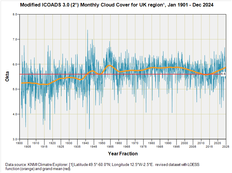
Now that is immensely satisfying! I feel a G&T coming on; maybe two…

I’ve not plonked a linear trendline down because I want to make a point with that orange wiggly LOESS function that there some twists and turns about the grand mean of 5.6 okta that point to cyclical and long-term processes. Alarmists are not keen on admitting to these for some reason; it is as though they’ve wooden rulers shoved up their jacksies. But hey, I’m happy to oblige with the linear thinking thing and can report a statistically significant positive trend of +0.045 okta per decade (p<0.001). Purists worried about serial correlation may wish to note the maximum likelihood estimate of +0.045 okta per decade (p<0.001). Yes, I’m being a cheeky monkey!

I think it’s time to slurp that drinkypoo. Until next time…

Kettle On!