A Modest Cloud Cover Study (part 3)

Today I have a stab at modelling the ICOADS v3 cloud cover dataset using the spanner that is ARIMA

Before I launch into time series modelling I’d like to take a closer look at the strange kink in the ICOADS v3 monthly cloud cover dataset for the study region. Here it is zoomed in a little with a couple of markers to assist our eyeballs:

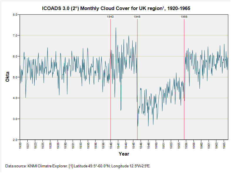
Those abrupt changes in 1945 and 1956 are unlikely to be anything other than disruption to the data collection regime arising from the impact of WWII in various ways. It’s curious that the impact of the war should linger as late as 1956 but, hey, rationing didn’t formally cease until 1954!

Being of a particularly suspicious mind set this morning I also plonked down a marker at 1940, for there appears to be a bit of a bump between then and 1945. Trouble is we’ll never know if this was a change in the weather or a change in the observation station sample for I’m guessing that northerly outposts were established to monitor wartime activities on the North Sea.

These bumps and lumps are a right pain for anybody wanting to use the ICOADS dataset as a time series so I thought I’d roll out my ARIMA spanner and have a go at predicting what the period 1940 – 1945 might have looked like using the historic data from 1853 – 1939. This may sound like a strange approach but this trick of self-prediction lies at the heart of much hefty ARIMA-based analysis that has been rolled out over the last few decades by the high and mighty.

Autocorrelation: Getting A Time Series To Predict Itself

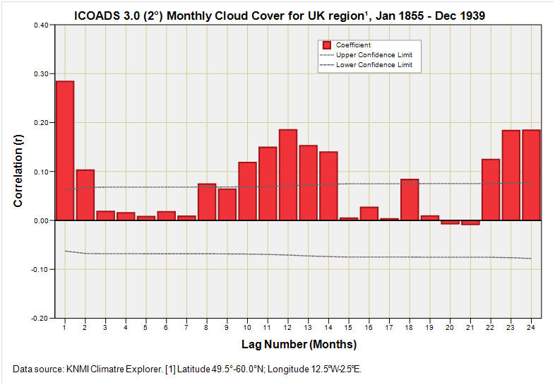
Self-prediction works well when there’s a great deal of autocorrelation within the time series (‘auto’ being derived from the Greek for ‘self’). So let’s take a look at an autocorrelation function plot:

There we go!

That big red bar sticking up above the upper 95% confidence limit at lag number 1 with a Pearson correlation of r = 0.284 tells us that if it was cloudy last month it is likely to be cloudy again this month, though this isn’t a strong correlation. Equally, therefore, if it was clear skies last month then it’s likely to be clear skies again this month (two horns on the same goat and all that).

See that surge in bars around the 12-month and 24-month lag positions? That there is seasonal stuff and this is telling us that cloudiness over the UK and Ireland is a seasonal thing, though the correlation is quite weak, peaking at r = 0.185.

So, then, we’ve got seasonality and we’ve got some sort of month-on-month memory effect. This makes total sense and is what we generally experience as UK & Eire land lubbers. The buzzword is autocorrelation and it means there’s going to be sufficient periodic structure in the ICOADS time series for ARIMA to get its teeth into. In turn this points to the likelihood of a reasonable predictive model coming out of the oven when I turn the handle.

ICOADS Monthly Cloud Cover Jan 1855 – Dec 1939

I guess we better start by taking a look at this historic time series in the flesh. Here it is with the series grand mean of 5.13 okta marked by a red line:

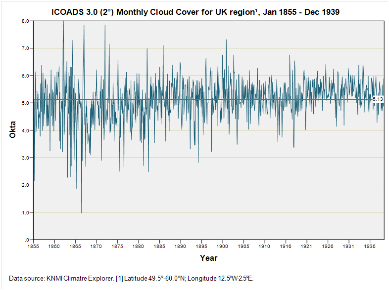
OK, so I typed okra there to begin with; a Freudian mistake, I suspect, coz it’s 12:09 BST and I’m thinking about food; and Mrs Dee is cooking-up something in the kitchen below that smells yummy! Heteroscedasticity would appear to be a feature of this time series with wild variation in values settling down over time. It’s impossible to determine whether this is due to a changing climate or the changing nature of the methodology. Please remember this mighty powerful and ever-present confounding factor next time you see an authority vomit something institutionally inane.

My eyeballs suggest a possible positive slope but they could easily be deceived by the heteroscedastic nature of the beast. That being said, a quick and dirty linear regression proffered a statistically significant slope estimated at +0.078 okta per decade (p<0.001). Don’t wait up.

Purists will want to see appropriate adjustment for serial correlation (a.k.a. autocorrelation) such as Cochrane-Orcutt or Prais-Winsten estimation, so I’ve gone and used a maximum likelihood spanner, this being a hot and fashionable tool these days. A good thing I did too, for the estimate of serial correlation (rho) fetched-up at ρ = 0.235 (p<0.001), and when accounted for this provided a clouding rate estimate of +0.078 okta per decade (p<0.001). Sometimes purists need a right good slap with a wet haddock to wake them from their anal dream.

Of greater interest to me is the wiggliness about that grand mean for it feels a tad periodic but, alas, I don’t have sufficient data points to dig deep into this using the spanner that is spectral analysis.

N.B. Some keen readers may ask why I started the series in January of 1855 instead of January of 1853 and the answer is… missing values that are too numerous to paper over.

ARIMA Model to Predict 1940 - 1960

I hope everybody understands what I’m doing here… I’m using the period January 1855 – December 1939 to predict values for the period January 1940 – December 1960 using the spanner that is ARIMA. There’s periodic behaviour within the data so hopefully we’ll get to see some useful predictions.

Using ‘expert’ mode the stats package settled on an ARIMA(0,0,8)(1,0,1) model structure which tells us a few things. First up we note a couple of zeros in the middle of each bracket pair; these denote the order of differencing. Thus, no non-seasonal differencing (d=0) and no seasonal differencing (D=0) was required and this situation arises if the time series is not gradually incrementing in value over time. In plain English cloud cover is pretty much what it has always been over the period 1855 – 1939: a feature witnessed by the flimsy regression results.

Second up we may note a good lump of the action sits in the second set of brackets that denote seasonal effects. In this regard we have a value of P=1 and Q=1 denoting first order seasonal autoregressive (AR1) and first order seasonal moving average (MA1) terms. This should not surprise us because it’s what we saw back in the autocorrelation function plot. In plain English the best-fitting cloud cover model contains seasonal components. Good gear!

The curious feature for me is that q=8 non-seasonal moving average term in the first pair of brackets. This tells us that the model wants to know what has been going on in terms of variation of cloud cover over the past 8 months before it makes a stab at guessing cover for this month. I’m guessing that this is something to do with conditions developing at sea, and the North Atlantic in particular. So let’s have a look at some tables:

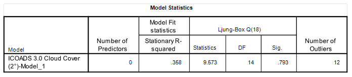
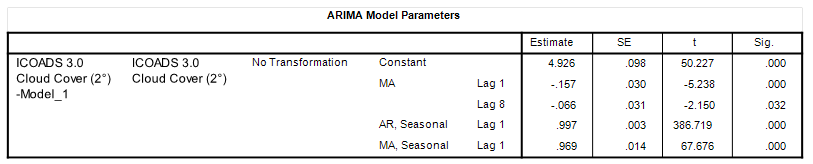
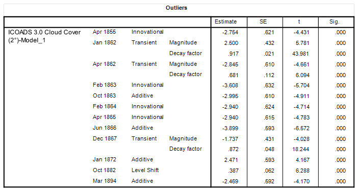
With a stationary R-square of 0.358 the model isn’t a great fit but then again who can guess the weather with any degree of accuracy? I think the most interesting table here is that for the outliers for we find a whole bunch of wacko values prior to 1900. This doesn’t fill me with confidence and I am tempted to re-model the data from 1901 onwards, this having the advantage of permitting me to use the CRU TS4.08 data as an independent (predictor) variable. But let us first look at the model in the crayoned flesh, so as to speak…

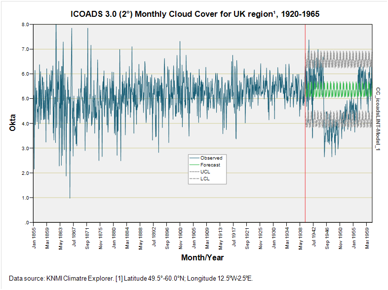
Now that is a terribly boring result lacking any flavour! We’ve been swindled!

The model has picked-up on the seasonality and is offering little else. Time to open the biscuits and have a think, methinks… and come back with something more exciting next time for we are now at the email limit once more.

Kettle On!